] add https://github.com/JuliaTDA/GeometricDatasets.jl
] add https://github.com/JuliaTDA/ToMATo.jlGetting started
Installation
In Julia, type
First usage
Load some libraries
using ToMATo
import GeometricDatasets as gd
using AlgebraOfGraphics
then define X as the following pointcloud with ds as density function:
X = hcat(randn(2, 800), randn(2, 800) .+ 4)
k = x -> exp(-(x / 2)^2)
ds = gd.Filters.density(X, kernel_function = X -> X .|> k |> sum)

df = (x1 = X[1, :], x2 = X[2, :], ds = ds)
plt = data(df) * mapping(:x1, :x2, color = :ds)
draw(plt)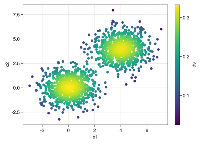
Then calculate its proximity graph
g = proximity_graph(X, 0.2, max_k_ball = 6, k_nn = 4, min_k_ball = 2)

fig, ax, plt = graph_plot(X, g, ds)
fig
┌ Warning: Axis got passed, but also axis attributes. Ignoring axis attributes (type = Makie.Axis, width = 600, height = 600).
└ @ AlgebraOfGraphics ~/.julia/packages/AlgebraOfGraphics/yhdjr/src/draw.jl:19
After that, we need to apply the ToMATo algorithm twice: the first time to estimate the parameter by analyzing the births and deaths of the connected components:
clusters, births_and_deaths = tomato(X, g, ds, Inf)

plot_births_and_deaths(births_and_deaths)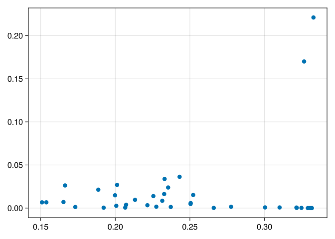
We can see that 0.1 is a reasonable cut for the peaks. Let’s calculate ToMATo again and plot it
τ = 0.1
clusters, births_and_deaths = tomato(X, g, ds, τ, max_cluster_height = τ)

fig, ax, plt = graph_plot(X, g, clusters .|> string)
fig
┌ Warning: Axis got passed, but also axis attributes. Ignoring axis attributes (type = Makie.Axis, width = 600, height = 600).
└ @ AlgebraOfGraphics ~/.julia/packages/AlgebraOfGraphics/yhdjr/src/draw.jl:19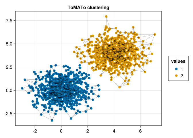
See the Examples section for more.